Code found here. I worked hand in hand with Tristan Frizza on this.
- Introduction
- What took us so long?
- Demonstrating robustness
- Learning from pixels
- Whats next?
- Appendix
Introduction
This is part of an ongoing series where Tristan and I are trying to re-implement the Learning from play (LFP) line of research, then build on it to answer a couple of questions, first of all:
“Can we enable fast transfer learning to new scenes or behaviours by using language to structure a joint trajectory embedding space between robot specific data and a much larger, diverse set of human video?”
We’ve finally nailed a great baseline re-implementation. In the gif above you can see goals specified by the transparent copies of the object - it is capable of reliably completing > 10 different tasks in a row. You can read a little bit more about their papers, the question we are trying to answer and getting the environment right in Laying down the infrastructure. The architecture is explained clearly in their papers, and we cover the main ideas in our previous post, so look to those resources if the work is unfamiliar.
What took us so long?
Once again - the answer wasn’t in neat regularisation techniques, interesting rotation representations, proprioceptive features, learnt initialisations for the LSTM or any of the other highly specific things we tried in response to particular deficiencies - it lay in more fundamental fixes:
- Realising how our ‘play’ was biasing the dataset
- Venturing beyond the plateau in our training curves,
- Understanding how to diagnose overregularisation
Learning to play again
I once heard that it takes abstract artists years to re-learn how to paint with the freedom and creativity of a child - it certainly took us months to learn how to ‘play’.
Take a look at this side by side comparison of the original paper’s teleoperated ‘play’, and our initial dataset. While we did both perform a similar diversity of tasks, they interact with objects more times in a row. We typically performed one interaction then moved to the next. What this meant is that a bias was burned in to immediately transition to another object following an attempted behaviour. Worse - if we weren’t careful in teleoperating then there were regular patterns in how we moved (it is very tempting to push the button after the door).

This can be bandaged over by shortening the re-plan interval - but our preference is for a model where the bias is ‘fix up the object you just interacted with’. Recollecting the data in this multi-interaction way dramatically improves how robust and accurate the model is. The ‘post interaction’ phase of a plan initialises the next plan with an ideal starting point for retrying (on failure), or fixing up (on partial success).
To verify that this effect was due to the the behaviour demonstrated, and not that a multi-interaction dataset provides more timesteps of interaction with the environment - we counted the proportion of timesteps where an environment variable was different to the previous state (i.e, arm interacting not transitioning), but the difference was negligible.
Diagnosing Overregularisation
Recall that there are two potential latent vector inputs to the actor.
- The output of the encoder over a trajectory, representing the specific path taken from A-B in the sampled trajectory
- The output of the planner when given only the initial state and the goal state, representing one potential path from A-B.
During training:
- The actor is trained to reconstruct the true actions over a trajectory using the encoder’s outputs, the state at each step of the trajectory, and the goal state
- The KL divergence between the encoder and planner’s outputs is minimised
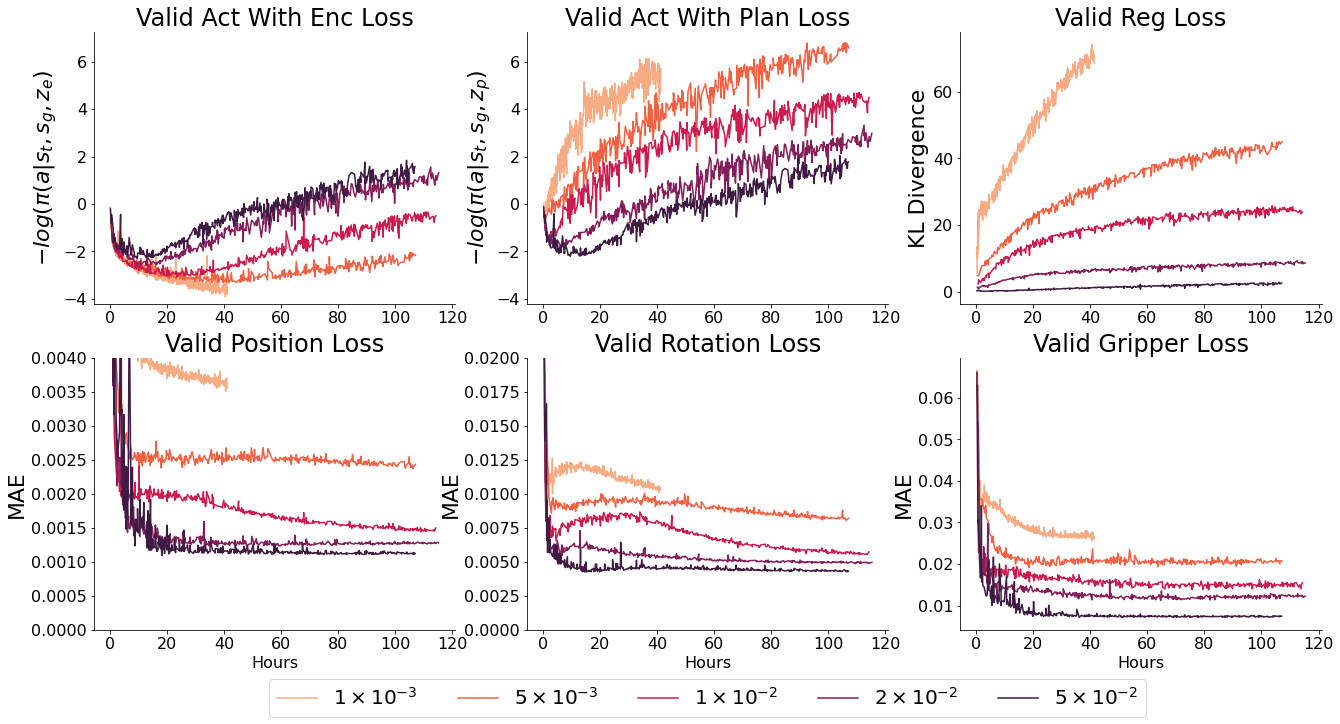
- $ \beta $ controls the weighting between KL divergence and action reconstruction loss. Too high, and the encoder is constrained to the planner. As a result, the latent space is uninformative and ‘acts with encodings’ loss will be worse, which limits the upper bound of performance by the model. Too low, and the planner is unable to catch up to and plan over the latent space created by the encoder - as a result the planner’s outputs will be unfamiliar inputs for the actor
At test time:
- The planner samples a potential ‘latent plan’, from which the actor constructs a trajectory.
- This may not be the path which was chosen in the demonstration (as there are many valid ways of accomplishing goals)
What this means is that training this model is a delicate balance between over and under regularisation. Neither the ‘reconstruction loss from encodings’ or ‘reconstruction loss from plans’ is a perfect guide to this, as overregularised models appear to converge to similar or better final values as well regularised models with informative latent spaces (but much faster - which would initially appear better).
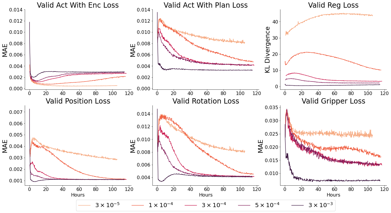
When deployed, over-regularised models perform noticeably worse - they do not handle the multimodality of the behaviour space as well. This is the commonly seen ‘blurry’ faces problem from older VAE architectures on images, they simply output mean values which do fine on a loss graph, but poorly as an output.
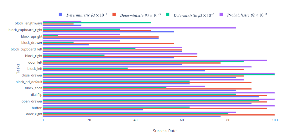
To quantify this, we defined a couple of standard tasks and measured the success rate of each model. Success is defined by placing all elements of the state within 5cm and 30 degrees of their goal position and orientation, or when the switch is flipped in the case of the dial and button. This is a reasonably restrictive goal - and fails to account for behaviour which is mostly correct. E.g. if it places the block in the cupboard or drawer in the wrong orientation it fails. Adjusting for this would bring the success rate of these tasks to ~85%. In addition, the robot only receives 4s to complete each task - given unlimited time the success rate is >90% for most tasks except placing the object in the drawer (where it runs the risk of knocking the block out of reach). Chaining goals is easier than these success rates would suggest - once the block is grasped subsequent block goals have > 90% success rate, it is the initial grasp which is tough - and sequential goals have higher probability of success than a cold start. However as these goals are entirely arbitrary, and ultimately that level of specificity and speed will be desirable with asymmetric objects - we think it suffices as a relative comparison.
The over regularised model (B0.0003) which has the best overall MAE reconstruction error performs universally worse than the optimally regularised models (B0.00003 or Probabilistic B0.02) because it displays classic symptoms of being unable to handle multimodality. Without fail it tries to randomly interact with other objects on it’s way to the goal - often shifting them far enough that the goal state is unsatisfied. It’s behaviour reveals a further dataset bias towards playing with the block over other objects. This is why it fails catastrophically at button pressing - a less frequent task in the dataset, but an easy enough task that models with a distinct representation succeed 100% of the time.
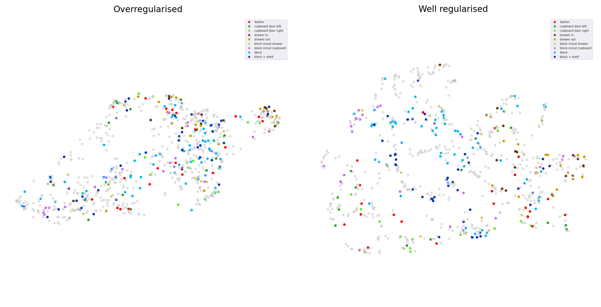
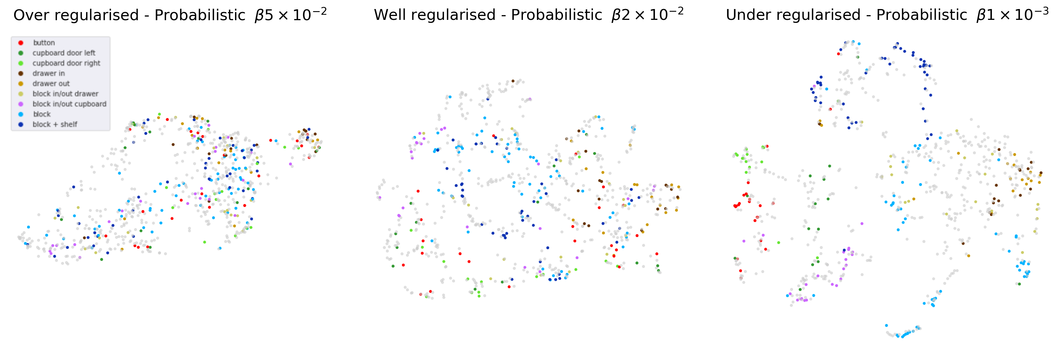
Evaluating training runs is therefore a mix of ensuring the action reconstruction loss converges to the best observed values - while using low enough $ \beta $ values that the latent space is distinct. The pattern of ‘reconstruction loss from plans’ should follow that of the regularisation loss, worse initially, then better as the space becomes informative - then plannable. One of the best ways to diagnose overregularisation is to label a set of trajectories with descriptions and plot their arrangement in latent space over the course of training. The latent space should become distinct quite early - and stay that way.
This is frustratingly qualitative. We were hoping that the encoder and planner reconstruction losses would converge to a lower final value for the well regularised models, even if the planner improved more slowly than for over regularised models - but this wasn’t the case.
Ultimately, the probabilistic and deterministic actor perform similarly - but the latent space of a similar probabilistic actor is significantly more expressive, perhaps because it captures the low level multimodality itself. As a result, we will use the probabilistic model going forward.
What lies beyond the plateau?
This one is a little obvious in retrospect. Train longer! Initially we used Colab TPUs for all of our training, and it just so happens that the point at which we break away from the plateau is just after the typical timeout. It always felt more important to try another experiment instead of restarting the old one - and our intuition didn’t account for the idea that 10 hours on a TPU might not be enough for the model to hit its stride. We didn’t see that the regularisation loss leveling off was in anticipation of it decreasing and bringing in the ‘act with plan’ loss (explained later).

This is compounded by the fact that there is a relatively narrow range of Beta values (the relative weighting between the regularisation term and the action reconstruction term) which work. Too high, and the latent space collapses. Too low, and it would take even longer than it did for the regularisation loss to bend down and allow the planned trajectories to match up to the encoded ones.
Demonstrating robustness
We could have done this more rigorously - but we wanted to keep progressing. Besides, isn’t kinetic punishment the fastest way to a robot’s heart? Its worth noting that there are a couple examples of picking the block off the floor in the play dataset - but only around ~5-10! It would be interesting to test whether similar behaviour emerged with no floor examples, only the differing height of the shelf, table and drawer interior.

Learning from pixels
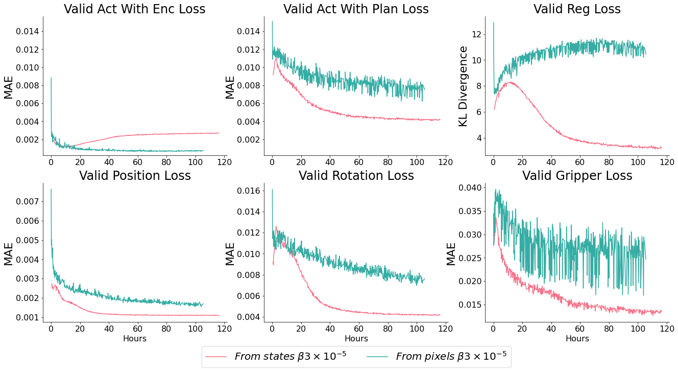
Our test run using pixels showed promising reconstruction loss decrease - but poor latent space convergence and end-task performance. It is clear that the encoder has sufficient capacity to memorise (it’s loss term tracks with the model which learns from states), but the planner may need increased capacity to be able to plan over the space, $ \beta $ may need to be increased to bring the spaces together - or it may need to be trained for longer (as we see the beginning of the slope off pattern).
We’d like to avoid different $ \beta $ values for states and images - as the reconstruction and regularisation magnitudes should be the same, which means their relative weighting should be the same too.
Whats next?
First up, we refactored the code so that it is an easy, extensible library for us to build on. We’re taking the time to explore engineering fixes which might speed up our iteration cycle (e.g, deep diving into TPU utilisation and trialling FP16). We’ve also decided to take a breather and improve the environment - we’re about a week from recreating the environment in Unity - mostly as a reward and a bit of fun, partly as a forcing function to set up conditions closer to a real robot. In particular, the env needs to be asynchronous with the commands sent.
By the time these fixes are done, we’re hoping a few good models have been trained from pixels - and we’ll recollect data, label a few thousand trajectories and re-implement Lang-LMP in our new environment. After that, we’ll finally be ready to begin asking questions! At last the pace is accelerating!
In addition to our primary question, we’re going to sidetrack slightly to check whether discrete VAEs can lead to improvements. Focusing on two things:
- Composing plans as a sequence of quantised latent vectors like VQ-VAE represents images as a sequence of quantised tiles - we think this may lead to a valuable decomposition of parts of skills, e.g sharing grasp encodings between objects or parts of the environment. Best of all - it would mean no more trade-offs with the planner ‘prior’, which would be learnt as a second stage
- Using VQ-VAE as a pretrained feature encoder for images: the 32x32 breakdown might work well for an object centric scene breakdown - in the same way which spatial softmax does.
For now, a little more engineering work! Here’s a teaser of the unity env - unfortunately hand tracking just wasn’t accurate enough - so controllers it was!

Thank you to Corey Lynch, Suraj Nair and Eric Jang for patiently answering our questions - and to the TFRC team for their support.
Appendix
Beta sweep of probabilistic models
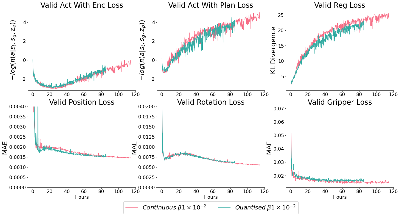
Comparison of quantised vs continuous action distributions
Comparison of deterministic vs probabilistic actors

Over vs well regularised latent spaces