Recently I found a way to learn state representations such that linear interpolation between the latent representations of states provided near optimal trajectories between the states in the original set of dimensions. They are learnt by optimising the representations of expert trajectories to lie along lines in higher dimensional latent space. The hard problem of finding the best path between states is reduced to the simple problem of taking a straight line between the latent representations of states - and the complexity is wrapped in the mapping to and from the latent space. This even worked for image based object manipulation tasks, and might be an interesting way to approach sub-goal generation for temporally extended manipulation tasks or provide a dense reward metric where latent Euclidean distance is a ‘true’ measure of progress towards the goal state.

I used two testing environments, my own testing environment where the gold point mass must push the red block to a goal positions https://github.com/sholtodouglas/pointMass and RLBench tasks.

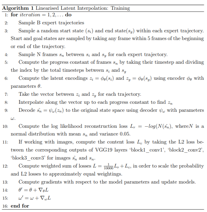
The image below depicts the intuition of the method, where states or images are transformed to latent representations (here reduced to 2D using UMAP) - then a straight line path gives the correct path when mapped back to the original problem space.

Here is the same method applied to a significantly more difficult problem, hallucinating a reasonable trajectory in image space for an unseen arrangement of the BBQ and meat in an RLBench Task.

Whilst it does display attractive properties as a reward function and hallucinate visually superb sub-goals and trajectories, when the representations are used agents are capable of finding local reward minima to exploit instead of solving the task. However, I thought it might be of interest that the latent space can be structured in this way - whether as the inspiration for future work, a sign not to pursue this path or just as a curiosity!

If this terminology is familiar, skip to the next section where I’ll outline current work on state representation learning and how this fits in. Otherwise, lets get some background.

What is State Representation learning?

A state is a vector where each dimension describes one aspect of the scene. In the example of robotic manipulation, the state could be made up of the positions, velocities and orientations of the gripper and the relevant objects – simple manipulation problems can be defined in under 20 dimensions. Modern reinforcement learning algorithms quickly begin to struggle as the dimension of problems increases – and this problem is exacerbated when working from images, which are effectively comprised of hundreds of thousands of dimensions.

Representations are transformations of the input data into a different vector which make it easier to solve downstream tasks. For example, the compressed representations output by the later layers of CNNs summarize the high level features of an image. The representations learnt by supervised learning on image classification tasks are excellent for transfer learning to other similar tasks, but are of limited use for robotic manipulation which requires different information such as the spatial relationship between objects. These requirements led to adjustments like the spatial softmax , which forces the representation to retain spatial information.

State representation learning is the study of explicitly engineering representations useful for control of the state in downstream tasks like manipulation. This often involves generative models such as Variational Autoencoders, which are comprehensively explained at Lil'Log

Themes in the Research

The first theme is to use the distance (typically Euclidean) between the latent representations of states as a better reward function for reinforcement learning or as a loss function for imitation learning. This avoids the difficulty of hand designing complex and failure prone dense reward functions, and allows for a better similarity metric between frames. Srinivas et al learn representations useful for planning and imitating a set of expert demonstrations while Ghosh et al use the difference in the actions used to reach states with a pretrained policy as a proxy for distance between states. Both approaches learn a representation for states which enables faster learning of new policies. Sermanet et al use contrastive losses to build viewpoint invariant representations by drawing frames from the same timestep but different viewpoints together. This worked excellently as a distance measure for imitation learning. All these approaches require either a selection of human tele-operated expert trajectories, or a pretrained goal conditioned policy to collect expert trajectories with.

The second theme is to use the latent space to make it easier to plan trajectories to reach goal states. Typically because it is faster and easier to simulate or optimize in the lower dimensional latent space than the original image space – allowing effective sub-goal generation , trajectory optimisation via Model Predictive Control or training of RL agents on simulated data . A particularly interesting paper by Watter et al structure the latent space so that successive states are a linear function of the current state and action, which allows the use of trajectory optimisation algorithms from optimal control such as LQR to be used. All of the above approaches are relatively computationally intensive, requiring significant simulation of many possible trajectories or reasonably complex optimisation in the latent space – but they can all be learnt in a fully self supervised way from any transitions.

I wondered if it would be possible to structure the state representations so that finding the best trajectory between two states was the easiest possible problem – that of taking a straight line between their latent representations. This would make it far less computationally intensive to find sub-goals for long horizon manipulation tasks and also function as a distance metric which uses progress towards the goal as a proxy for distance between states - which could be a better proxy than the others studied.

I thought it might be possible to force points along expert trajectories to lie along lines in latent space if the dimension was higher than the intrinsic dimension of the state (the minimum number of dimensions required to represent the state), based on the fact that SVMs are able to find linearly separable boundaries between points when transformed to higher dimensions using the kernel trick. The higher dimension isn’t an issue when working with images as the difference between latent vector sizes in marginal. As it turns out, this was already a familiar concept in control theory called the 'Koopman Operator'. Lusch et al use a very similar approach to model nonlinear systems linearly by mapping states to a higher dimensional representations which are eigenvectors of a learnt transition operator K. Recall that the multiplication of an matrix by it's eigenvector gives a scalar mutliple of the eigenvector, and so all states of a system vary along a straight line in latent space.

Method

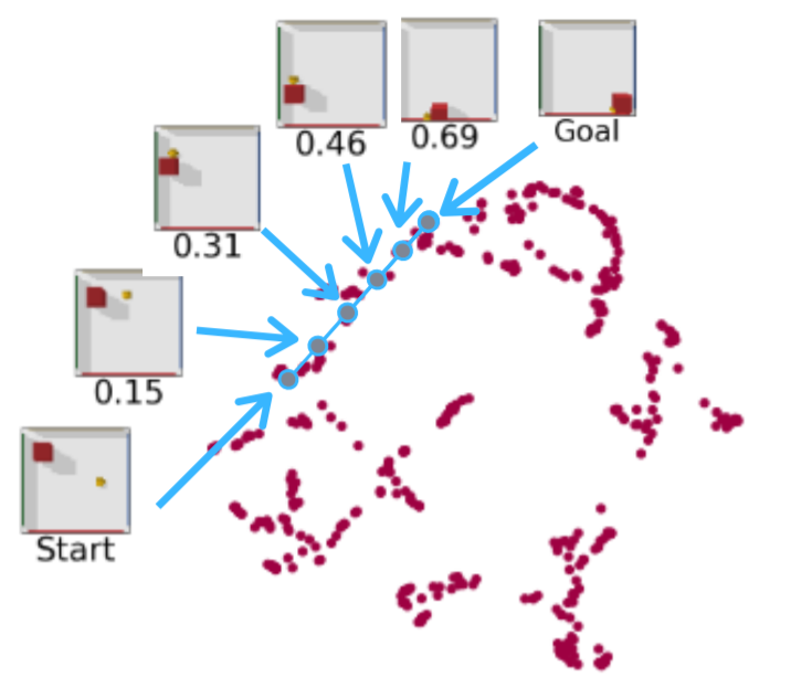
Take two random frames from an expert trajectory as a start (s_i) and end state (s_g), and encode into latent variables (z_i, z_g) with a network that functions as the encoder of a VAE. Sample the frames between them and interpolate between (z_i, z_g) proportionately to the number of timesteps away each frame is. Using another network as a decoder of the VAE, decode these interpolated variables and compute the reconstruction loss with the sampled intermediate frames. Backpropogate through the decode, interpolation and encdoer and the VAE learns to jointly encode/reconstruct and enforce that the points lie along the interpolated path in latent space with a single loss term.

Training of the VAE using an expert trajectory from the point mass task.

Interpolation between latent transformations mapped back to state space showing a valid trajectory.

Earlier, when I tried a separate reconstruction loss and a linearization loss by taking the distance between the latent encodings of generated frames along a trajectory to the line between z_i, z_g, it failed to work because balancing the weightings of reconstruction and linearization loss was extremely difficult. Additionally, in order to get it to work on images, content loss had to be used in addition to pixelwise loss as the reconstruction loss.

To use it to plan trajectories, simply encode any pair of start and end goal states, interpolate between them and decode along the path. To use it as a reward function, simply encode and take the L2 distance between frames.

Results

Multi-task Embeddings

Like all the methods from the first theme of research, this method does not learn exlcusively from the transitions experienced during a policy's random exploration and requires a degree of supervision. As a result, it would be most useful if it could be pretrained on large datasets of video of various tasks being completed (which is much easier to collect and generalize than teleoperation data) - and then used as a baseline embedding which could be transfer learned to new tasks with a handful of task specific demonstrations. 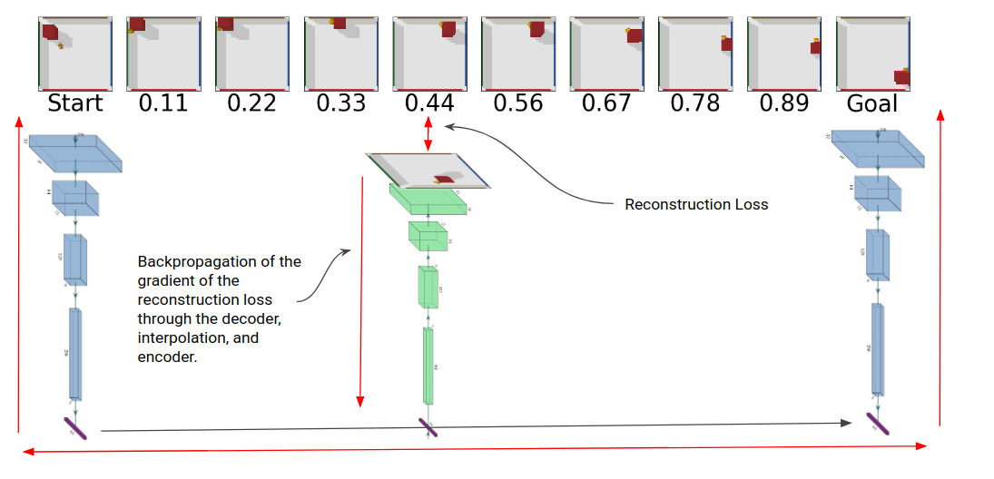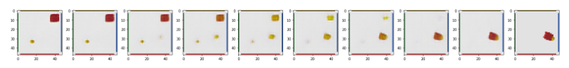As an inital test of this, the same model was trained on 3 tasks from RLBench , the dish placement, oven opening and BBQ grilling tasks. Each tasks has 3 viewpoints, the left and right shoulder cameras and the gripper camera. The model achieves some amount of success here, clearly hallcuinating reasonable intermediate frames for use as sub-goals inclduing the changing viewpoint of the gripper.

Generated intermediate frames on the dish, oven and grill tasks, the limited data on the dish task affects reconstruction quality, but on all viewpoints the gripper decoder clearly learns the concept and timing of required grasps and hallucinates them appropriately.

Comparison with the Latent Space of a Standard VAE

To highlight the difference between the properties of the latent space constructed by a standard variational autoencoder and this one, observe the stark difference in interpolation between the following two images on the pointmass task. With a standard variational autoencoder, the interpolation between the embeddings of two states does gradually change between the two images, but the interpolation is physically infeasible. By contrast, interpolation in a linear latent space shows a valid path between two new images.

A standard VAE trained on images, without linear structure in the latent space. Interpolation between the start and end state is physically infeasible and thus states which are close in the latent space do not correspond to progress.

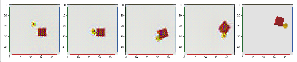
Successful image based model with a linearised latent space.

Latent Distance as an Effective Reward Metric

L2 distance in the latent space should correspond to the true distance between a state and a goal. With a linearly structured latent space the latent distance decreases throughout the entire trajectory, providing a clear reward landscape to follow. By contrast, the standard VAE and the pixel-wise distance are a strong measure in the final frames of a trajectory, once it is very close to the goal image - but pre-contact it is a flat or increasing measure, and as a result it would be extremely difficult for an agent to escape the reward plateau.

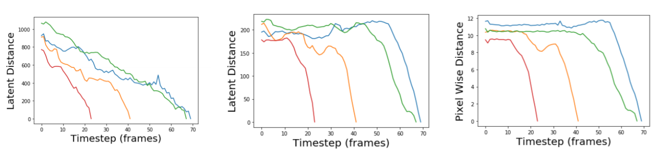
For a sample of expert trajectories, each in a different color, the latent distance between the embedding of each frame with the goal with an autoencoder with linearised latent space, a standard autoencoder, and the pixel-wise distance between the original frame and the goal image is compared from left to right.

Unfortunately, in experiments with using the latent distance as a reward metric - the policy still seemed to be able to find local minima to exploit, and this remains an unsolved issue with the method.

Working in High Dimensions

As the dimensionality of space increases, the density of points uniformly distributed throughout the volume of the space will cluster in a thin shell on a hypersphere (a set of points at constant distance from the origin) in that set of dimensions. This contradicts lower dimensional intuition, which suggests points are more uniformly distributed throughout the space. This means that linear interpolation between points in high dimensions will typically traverse regions of space with very low probability density and so a generative model (like our VAE) will struggle to reconstruct them. Kilcher et al demonstrated that spherical interpolation between points in high dimensions results in significantly better reconstruction with generative models.

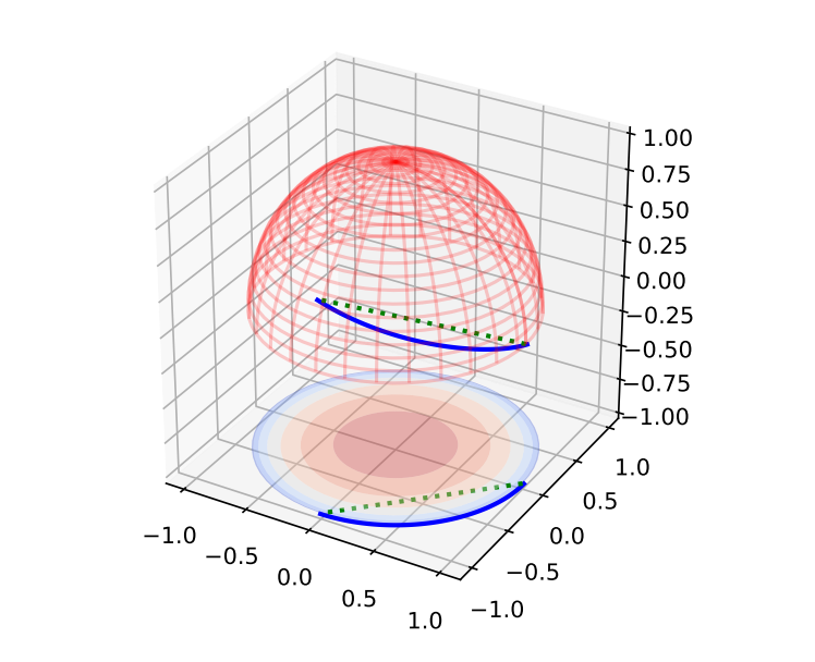
3D Visualisation of a hypersphere demonstrating that linear interpolation takes a path through regions of state space without many embeddings from which the model will not be trained to reconstruct, while spherical interpolation traverses familiar space.

I tested this and found that using spherical interpolation was only roughly as successful as linear interpolation. I hypothesized that when using linear interpolation, the method of jointly optimizing for reconstruction and interpolation spreads mass throughout the entire hypersphere - which means spherical interpolation was unnecessary. I tested this on the 64 dimensional encodings of images by sampling a batch of trajectories, calculating their vector magnitudes and centering them about the average vector magnitude. This gave an approximately normal distribution of values, indicating that the method spreads the density throughout the space normally instead of in a thin shell and thus linear interpolation is valid.

Moving forward, spherical interpolation makes significantly more sense because it allows for harmonic motion (where continuing will return the state to the original state) and allows for multimodal paths between states.

How Many Dimensions are Required?

Recall that the original hypothesis was that higher dimensions than the original state space would be required to model problems. To confirm this, reconstruction quality from interpolation through the latent space was tested for a set of different values for the dimensionality of the latent space. The simulation environment used was the point mass and block environment, as a result the observation vector size was 8 - containing the xy positions and velocities of both the mass and the block. The results indicate that the required set of dimensions is one higher than the intrinsic dimension of the problem, with decreasing returns on dimensionality after two higher. In this case, 4 dimensions are required to represent the positions of the mass and the block, and a 4 dimensional latent space fails to successfully linearize the space in terms of position. When represented in 5 or greater dimensions the quality of reconstruction increases significantly, but each additional dimension after the latent dimension exceeds the intrinsic dimension has a decreasing effect.

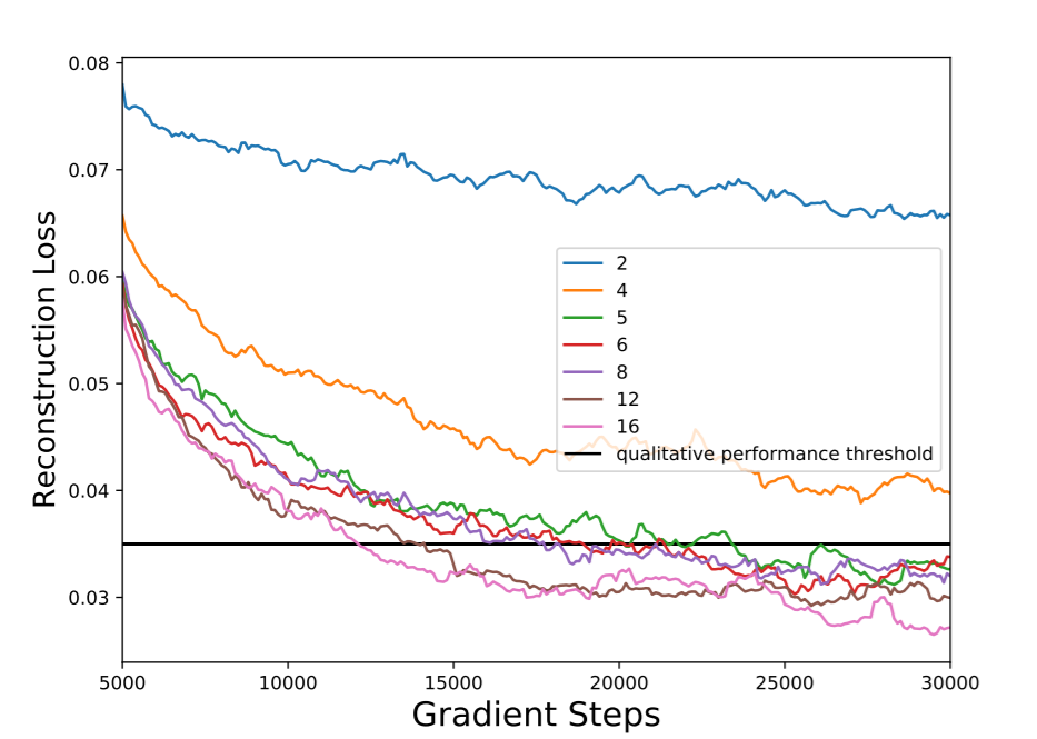
Reconstruction Loss for a range of latent dimensions exhibiting decreasing returns after the dimensions exceed the intrinsic dimension of 4 by two.

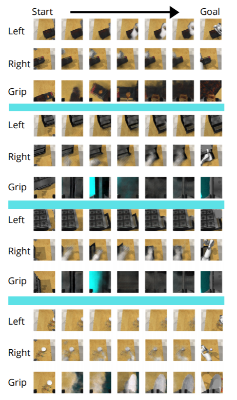
Algorithm and Architecture Specifics

Here is a more detailed breakdown of the training process. You can also find the (messy) code in the repo https://github.com/sholtodouglas/linearised_state_representations with architecture details.

Linearised State Representations for Reinforcement Learning