
Playing with Energy Models
I was inspired to look into energy models after Yann LeCun’s talk on energy based self supervised learning.
The gist is this - for a given input $x$, an energy model $F(x)$ outputs a single value. We train it so that $x$ of the kind we’d like to generate is given low values, and everything else is given high values. This means we can start off with a random input, and use the energy model to give us feedback about how to tune it into something like what we want by taking the gradient of the output value with respect to the input.
Energy models offer a way to train a single generative model which is simpler to train than Generative Adversarial Nets (GANs) and more expressive than Variational Autoencoders (VAEs). VAEs typically require the use of reconstruction losses - which do not perform well on more complex generative tasks like images because per pixel reconstruction error is a poor proxy for overall image quality. GANs overcome this with the learned discriminator (and thus produce much better quality generated samples), but coordinating the adversarial training is extremely difficult - it is much easier to train the discriminator than the generator.
In the unconditional case, the goal is to train a function $F(x)$ which outputs a low scalar ‘energy’ value for inputs of the type we would like to generate (positive examples), and high for everything else (negative examples). This is very similar to training the discriminator of a GAN (which outputs the probability that a generated sample is real). A conditional energy function $F(x,y)$ outputs low energy for $(x,y)$ pairings which follow from eachother given our data. For example, $x$ and $y$ could be the coordinates of points on a spiral, or $x$ and $y$ could be successive frames in a video.
To generate using an unconditional energy function, you begin with $x$ as random noise, input this into the energy function, take the gradient with respect to the energy and minimise it by changing $x$. With conditonal models, you only change $y$ to minimise the energy. Repeat until convergence.
$ \hat{y} = \min_{y} F(x,y) $
Form of the energy function
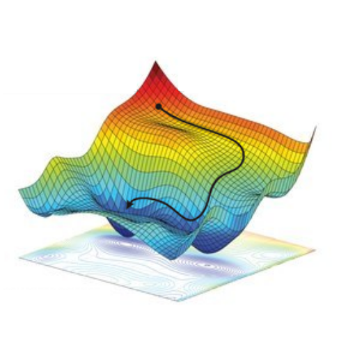
Traditionally, energy models have been formalised probabilistically, with the model outputting a distribution - and the training objective being to decrease the negative log likelihood of ‘low energy’ examples under this distribution, and vica-versa. In the video, Yann argues that using distributions won’t lead to as smooth an energy surface because the distribution will often be non probabilistic, “the distribution would be infinity on the [data] manifold, and 0 just outside it”. To model this properly will require infinite weights and give a ‘golf course’. What we want is a really smooth energy manifold to descend down, and probabilistic methods break that.
In the simplest form, the models are just a neural net with a single output node in the final layer representing the energy. To train this here is a whole taxonomy of potential methods, and in the video contrastive and architectural methods are highlighted.
Contrastive methods have a training objective that optimises the model such that $F(x_i , y_i)$ is strictly smaller than $F(x_i, y)$, where $x_i, y_i$ are paired examples, and $y$ are negative examples. Architectural methods restrict the informational capacity of the model, and include everything from PCA and K-means to sparse autoencoders which use a regularization term to limit the volume of space that has low energy.
Loss Function
One contrastive objective is margin ranking loss. If the energy of unpaired samples is greater than the paired samples, then the loss is 0. If the energy of paired samples is greater than unpaired samples, then the net loss will be positive. The margin value encourages a minimum difference between the energy of paired vs unpaired examples.
$ Loss = max(0, −( F(x_i, y) - F(x_i , y_i) )+ margin ) $
Predicting Under Uncertainty
Using latent variables allows us to recover the ability to predict under uncertainty. Without this, in stochastic environments like the real world, models will have blurry predictions that are an average of the possibilities rather than the most likely possiblity. By conditioning the energy model on a latent variable F(x,y,z), you can sample from the random vector z to introduce a degree of flexiblity into a nonprobabilistic EBM. Watch the video for more, as I am only dealing with deterministic environments in this post.
Choosing Negative Examples
The primary difficulty with the contrastive training of energy functions is choosing the negative examples. GANs use a generator to produce realistic outputs which fool the discriminator, energy functions need similarly difficult negative examples to train properly - in high dimensional spaces random samples are insufficient. This is solved by ‘hard negative mining’, which amongst other methods can be approached by using mismatched pairs from the dataset (for example, video frames which do not follow after one another), and using prioritizied sampling of frames to select the negative samples wrongly given low energy values by the model.
Results
As an initial test of the models, I created energy functions for simple 2D functions - like a spiral. Its extremely easy to verify correctness by visualising the energy of sampled points on a 2D plane. The energy function for a spiral is the most clear visualisation I’ve seen of the increased modelling capacity of a neural network as layer size increases. I used a 3 layer network with varying layer size, and the energy of a plane is shown below.
Sampling random points and decending the energy surface gives a reasonable distribution along the spiral - but even with as simple an object as this there are dips in the energy function where points overcollect. Ideally, all points along the spiral should have the same energy - but this is not directly optimised for.

Other examples include two intersecting parabolas.

Using Energy Models in Planning and Reinforcement Learning
Recently I also became interested in looking at combining planning and reinforcment learning, inspired by:
-
Hallucinative Topological Memory for Zero-Shot Visual Planning (HTM), which uses a conditional VAE to sample from possible states in the environment, measures the distance between all of them using a model trained on example expert trajectories, then uses graph search to find the shortest path between start state and goal. A lower level tries to reach each state along this shortest path as a series of sub-goals. The C-VAE is able to adapt to unseen environments from the same theme at test time.
-
Search on the Replay Buffer: Bridging Planning and Reinforcement Learning (SORB), instead of using a conditional VAE they sample from observed states in the replay buffer, and then measure the distance between them using the value function of the lower level (by taking the value of a state conditional on the other state as a goal). Similar graph search and lower level subgoal reaching follows.
I like these ideas as they break down long horizon problems into achievable subgoals and are highly interpretable. I prefer the use of the q or value functions from the lower level to measure distance between states as per SORB, as this does not require expert trajectories. However, I find the idea of randomly sampling from the replay buffer to find potential subgoals inefficient - and would prefer to only search on states likely to be between the current state and the goal.
By building off the C-VAE of HTM, I thought it might be possible to create a generative model which generated states likely to be between the states as opposed to from the environment generally. This could be done by using the trajectories collected during RL exploration, and training a model to generate the states in between observed states. These will not be generated in an optimal path - but thats what the graph search is for!
Generating States Along Trajectories with Energy Models
For this generative model, I decided to experiment with an energy model. My first experiments involved a trivial task - moving a pointmass to a goal position on a flat plane. This is not the kind of long horizon task where planning should help, but its critical to ensure it performs reasonably in a simple and interpretable task.
To train this, I trained a condtional energy model where $x$ was the current state and the goal, $y_+$ was points along trajectories, $y_-$ was randomly sampled states.
The model clearly learns to create an energy valley between the current state and the goal (represented by the red and blue dots). However, there is clearly a high energy saddle between them - this is likely because I sampled points randomly along the trajectories of the point mass - and it moves with highest velocity in the center, taking time to accelerate and decelerate. This means that points at either end will be overrepresented in the dataset.

Generating random points and then letting them descend the energy surface gives a reasonable sample of points along the path. By not continuing to convergence, we eliminate the issue of dips in energy at the ends of the trajectory and ensure reasonable coverage along the path.

Using the Q value function of a model trained to reach goal positions allowed me to measure the distance between states, and connect states into a shortest path between the start and end.

Conclusion
I found it interesting to do a set of quick experiments with energy functions for generating states to plan with, but my results were not very compelling. Firstly, the generated states didn’t include the direct straight line, optimal path - even in a very simple problem. Secondly, even spiral generation was flawed. EBMs have a lot of promise and have achieved extremely powerful results - but for my RL interests, I’m going to continue to experiment with other ideas rather than pursuing the path of trying to get this framework to work well.
Update
Yilun Du pointed me towards his paper https://arxiv.org/pdf/1909.06878.pdf, which is a great approach where they use the energy function to model the probability of state transitions $E(s_t, s_{t+1})$, then take the product of probabilities of an (initially random) sequence of states and then use the energy function to find the most likely sequence of states given the start and goal state. This is neat because it solves both the state generation and planning problem, while needing only random state transitions instead of full trajectories between states. This means that you can do active learning - trialling the trajectories generated and then updating the energy model if they were infeasible. If I come back to this, that is the work I will build off!